Robot and interface specifications
Realtime control commands sent to the robot should fulfill recommended and necessary conditions. Recommended conditions should be fulfilled to ensure optimal operation of the robot. If necessary conditions are not met then the motion will be aborted.
The final robot trajectory is the result of processing the user-specified trajectory ensuring
that recommended conditions are fulfilled. As long as necessary conditions are met, the robot
will try to follow the user-provided trajectory but it will only match the final trajectory
if it also fulfills recommended conditions. If the necessary conditions are violated, an error
will abort the motion: if, for instance, the first point of the user defined joint trajectory
is very different from robot start position (start_pose_invalid error
will abort the motion.
Values for the constants used in the equations below are shown in the Limits for Panda and Limits for Franka Research 3 section.
Joint trajectory requirements
Necessary conditions
Recommended conditions
At the beginning of the trajectory, the following conditions should be fulfilled:
At the end of the trajectory, the following conditions should be fulfilled:
Cartesian trajectory requirements
Necessary conditions
Conditions derived from inverse kinematics:
Recommended conditions
Conditions derived from inverse kinematics:
At the beginning of the trajectory, the following conditions should be fulfilled:
At the end of the trajectory, the following conditions should be fulfilled:
Controller requirements
Necessary conditions
Recommended conditions
At the beginning of the trajectory, the following conditions should be fulfilled:
Limits for Panda
Limits in the Cartesian space are as follows:
Name |
Translation |
Rotation |
Elbow |
|---|---|---|---|
1.7 |
2.5 |
2.1750 |
|
13.0 |
25.0 |
10.0 |
|
6500.0 |
12500.0 |
5000.0 |
Joint space limits are:
Name |
Joint 1 |
Joint 2 |
Joint 3 |
Joint 4 |
Joint 5 |
Joint 6 |
Joint 7 |
Unit |
|---|---|---|---|---|---|---|---|---|
2.8973 |
1.7628 |
2.8973 |
-0.0698 |
2.8973 |
3.7525 |
2.8973 |
||
-2.8973 |
-1.7628 |
-2.8973 |
-3.0718 |
-2.8973 |
-0.0175 |
-2.8973 |
||
2.1750 |
2.1750 |
2.1750 |
2.1750 |
2.6100 |
2.6100 |
2.6100 |
||
15 |
7.5 |
10 |
12.5 |
15 |
20 |
20 |
||
7500 |
3750 |
5000 |
6250 |
7500 |
10000 |
10000 |
||
87 |
87 |
87 |
87 |
12 |
12 |
12 |
||
1000 |
1000 |
1000 |
1000 |
1000 |
1000 |
1000 |
The arm can reach its maximum extension when joint 4 has angle
Limits for Franka Research 3
Limits in the Cartesian space are as follows:
Name |
Translation |
Rotation |
Elbow |
|---|---|---|---|
3.0 |
2.5 |
2.620 |
|
9.0 |
17.0 |
10.0 |
|
4500.0 |
8500.0 |
5000.0 |
Joint space limits are:
Name |
Joint 1 |
Joint 2 |
Joint 3 |
Joint 4 |
Joint 5 |
Joint 6 |
Joint 7 |
Unit |
|---|---|---|---|---|---|---|---|---|
2.7437 |
1.7837 |
2.9007 |
-0.1518 |
2.8065 |
4.5169 |
3.0159 |
||
-2.7437 |
-1.7837 |
-2.9007 |
-3.0421 |
-2.8065 |
0.5445 |
-3.0159 |
||
2.62 |
2.62 |
2.62 |
2.62 |
5.26 |
4.18 |
5.26 |
||
10 |
10 |
10 |
10 |
10 |
10 |
10 |
||
5000 |
5000 |
5000 |
5000 |
5000 |
5000 |
5000 |
||
87 |
87 |
87 |
87 |
12 |
12 |
12 |
||
1000 |
1000 |
1000 |
1000 |
1000 |
1000 |
1000 |
The arm can reach its maximum extension when joint 4 has angle
Important
Note that the maximum joint velocity depends on the joint position. The maximum and minimum joint velocities at a certain joint position are calculated as:


In order to avoid violating the safety joint velocity limits, the Max/Min Joint velocity limits for FCI are more restrictive than those provided in the Datasheet.
As most motion planners cannot deal with those functions for describing the velocity limits of each joint but they only deal with fixed velocity limits (rectangular limits), we are providing here a suggestion on which values to use for them.
In the figures below the system velocity limits are visualized by the red and blue thresholds while the suggested “position-velocity rectangular limits” are visualized in black.
 Velocity limits of Joint 1 |
 Velocity limits of Joint 2 |
 Velocity limits of Joint 3 |
 Velocity limits of Joint 4 |
 Velocity limits of Joint 5 |
 Velocity limits of Joint 6 |
 Velocity limits of Joint 7 |
Here are the parameters describing the suggested position-velocity rectangular limits:
Name |
Joint 1 |
Joint 2 |
Joint 3 |
Joint 4 |
Joint 5 |
Joint 6 |
Joint 7 |
Unit |
|---|---|---|---|---|---|---|---|---|
2.3093 |
1.5133 |
2.4937 |
-0.4461 |
2.4800 |
4.2094 |
2.6895 |
||
-2.3093 |
-1.5133 |
-2.4937 |
-2.7478 |
-2.4800 |
0.8521 |
-2.6895 |
||
2 |
1 |
1.5 |
1.25 |
3 |
1.5 |
3 |
Important
These limits are the values that are used by default in the rate limiter and in the URDF inside franka_ros. However, these are only a suggestion, you are free to define your own rectangles within the specification accordingly to your needs.
Since FR3 does not inherently implement any restriction to the system limits (red and blue line in the plots above), you are also free to implement your own motion generator to exploit the HW capabilities of FR3 beyond the rectangular limits imposed by existing motion generators.
Denavit–Hartenberg parameters
The Denavit–Hartenberg parameters for the Franka Research 3 kinematic chain are derived following Craig’s convention and are as follows:
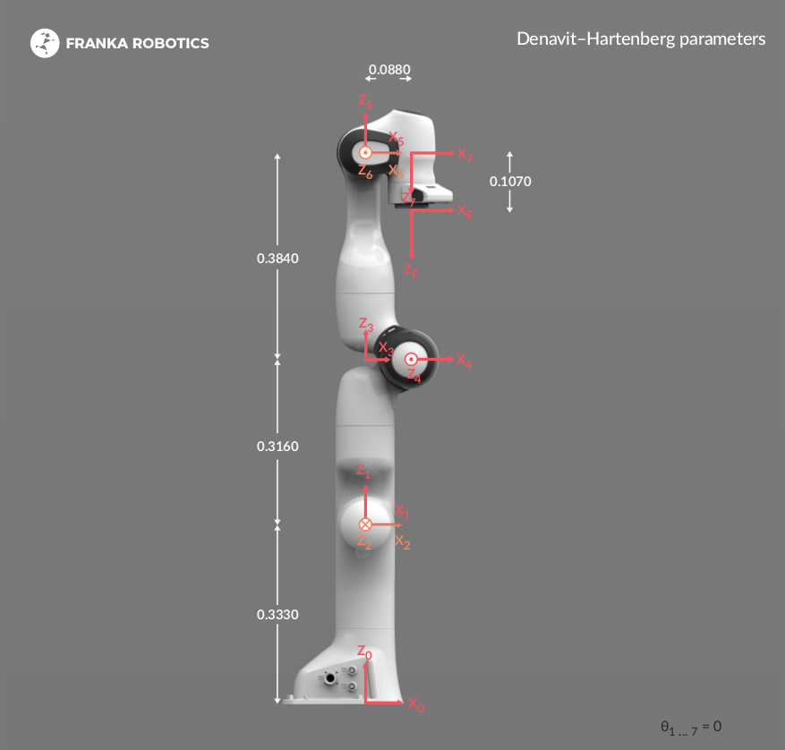
Franka Research 3 kinematic chain.
Joint |
||||
|---|---|---|---|---|
Joint 1 |
0 |
0.333 |
0 |
|
Joint 2 |
0 |
0 |
||
Joint 3 |
0 |
0.316 |
||
Joint 4 |
0.0825 |
0 |
||
Joint 5 |
-0.0825 |
0.384 |
||
Joint 6 |
0 |
0 |
||
Joint 7 |
0.088 |
0 |
||
Flange |
0 |
0.107 |
0 |
0 |
Note